Modeling extensible fibers in Cytosim
Author: Marco Pensalfini, UPC-BarcelonaTech, April 2022
Objective
This tutorial discusses a custom-implemented fiber class that allows modeling extensible fibers, e.g. intermediate filaments.
We will cover the theory and algorithms that underlie fiber modeling, the implementation of a stretchable fiber class in Cytosim, and finally some examples. The code is available on GitLab as part of Cytosim.
Preamble
According to Cytosim's documentation, fibers are modeled as inextensible along their longitudinal axis. Thus, to describe longitudinal extensibility, we will leverage Cytosim's ability to handle fiber growth. Specifically, at each time step, we will quantify the force acting on the fiber ends and adjust the length according to a prescribed constitutive behavior. We will discuss several alternative constitutive behavior for stretchable fibers, along with their potential limitations.
Theory and algorithms
Modeling an extensible fiber using Hooke's law
We consider an athermal system comprised of a straight fiber and two springs that connect the fiber ends to two points ($P$ and $Q$). The springs have elastic constant $k_s$ and the initial position of $P$ and $Q$ coincides with that of the fiber ends, so that $\overline{PQ}(0) = \ell(0) = \ell_0$. Thus, the spring elongation is initially zero: $\Delta u_s (0) = 0$. The fiber has initial length $\ell(0) = \ell_0$, cross-sectional area $A_f$, and it is made of a material with elastic modulus $E$, leading to the initial stiffness $k_f(0) = EA_f/\ell_0$.

To elongate the fiber, we gradually displace the points $P$ and $Q$ along the fiber longitudinal axis in $N$ identical steps until a final distance $\overline{PQ} (N) = L$ is reached. At each step:
- the distance $\overline{PQ}$ is increased by an amount $\Delta L = \frac{1}{N}\left[\,\overline{PQ}(N) - \overline{PQ}(0)\,\right] = \frac{1}{N}(L - \ell_0)$, reaching the current value $\overline{PQ}(i) = \ell_0 + i \Delta L$;
- the current extension of each spring is measured by $|\Delta u_s(i)|$, where $\Delta u_s(i) = \frac{1}{2}\,\left[\,\overline{PQ}(i) - \ell(i-1)\,\right]$;
- the spring extension causes a corresponding force acting on the fiber ends, $f(i) = k_s \Delta u_s(i)$;
- the force change in the current step ( $\Delta f(i) = f(i) - f(i-1)$ ) causes the fiber length to change by $\Delta \ell(i) = \Delta f(i)\,/\,k_f(i-1)$, where $k_f(i-1)= EA_f\,/\,\ell(i-1)$ is the last known fiber stiffness;
- per its definition, the current fiber strain is $\varepsilon(i) = \ell(i)\,/\,\ell_0 - 1$;
- the force acting on the fiber ends is obtained by cumulating the values of $\Delta f(j)$ occurred from $j=0$ to $j=i$, $F(i) = \sum_{j=0}^{i}\Delta f(j)$.
We implement the above algorithm in a Python function:
def ElasticFiber(ks, EAf, ell0, L, N):

    #initialize arrays
    PQ    = ell0 * np.ones(N+1)      #values of PQ distance at each step
    ell   = ell0 * np.ones(N+1)      #values of fiber length at each step
    du_s  = np.zeros(N+1)            #values of current spring extension at each step
    f     = np.zeros(N+1)            #values of force acting on fiber ends at each step
    df    = np.zeros(N+1)            #change in force values from previous to current step
    eps   = np.zeros(N+1)            #values of current fiber strain at each step

    #loop for load application
    for i in range(1,N+1):
        PQ[i]   = ell0 + i * (L - ell0) / N           #update current PQ distance
        du_s[i] = np.abs(PQ[i] - ell[i-1]) / 2.       #update current spring elongation
        f[i]    = ks * (PQ[i] - ell[i-1]) / 2.        #update current force at fiber ends
        df[i]   = f[i] - f[i-1]                       #update force change from previous to current step
        ell[i]  = df[i] / (EAf / ell[i-i]) + ell[i-1] #update fiber length after current step elongation
        eps[i]  = ell[i] / ell0 - 1.                  #update fiber strain after current step elongation

    F = np.cumsum(df)                #measure force during loading as cumulative sum of the df values

    #return results
    return PQ, du_s, ell, eps, F
We use this function to simulate a case where we want to reach $L = 2 \ell_0$ in $N=50$ steps for a system with $k_s = EA_f/\ell_0$:

Since the fiber and the two springs have comparable stiffness, they share the externally-applied deformation almost equally (hence the maximum value of $F/EA_f$ is around $1/3$). To have the fiber take most of the applied deformation, we need to increase the stiffness ratio $\gamma_0 = k_s \ell_0 / EA_f$.
Monitoring the fiber elongation $\Delta \ell(i)$ and the fiber force $F(i)$ at each step of the algorithm, we can observe that the force-strain curve is linear with slope $EA_f$ for any value of $\gamma_0$, but:
- values of $\gamma_0 < 2.0$ yield fiber elongations that are insufficient to bridge the distance between points $P$ and $Q$ ($\Delta \ell(i) < \Delta L$ $\forall i$); the share of applied deformation that is borne by the fiber increases for larger $\gamma_0$, in line with the expectation for a set of three springs in series (the fiber and the two connecting springs of stiffness $k_s$);
- for $\gamma_0 = 2.0$, the fiber elongation oscillates between the value $\Delta L$ and $0$; the oscillation is bounded and the fiber force keeps increasing throughout the algorithm steps;
- values of $\gamma_0 > 2.0$ result in an unbounded oscillating behavior both for $\Delta \ell(i)$ and $F(i)$, which diverge to infinity; this limits the maximum values of $\gamma_0$ that can be used in practice.

To understand the limitations in terms of admissible values of $\gamma_0$, we write explicitly the first few steps of the algorithm. The fiber elongation at the $i$-th step is:
$$\Delta \ell(i) = \frac{\Delta f(i)}{k_f(i)} = \frac{\ell(i-1)}{EA_f} \left[ f(i) - f(i-1) \right]$$Using the definitions of $f(i)$, $\Delta u_s(i)$, and $\overline{PQ}(i)$ given in steps #1$-$3 of the algorithm, it is immediate to show that:
$$\Delta \ell(i) = \ell(i) - \ell(i-1) = \gamma_0 \frac{\ell(i-1)}{2 \ell_0} \left[ \Delta L - \ell(i-1) + \ell(i-2) \right]$$For $i=1$, knowing that $\ell(-1) = \ell(0) = \ell_0$, this results in:
For $i=2$, we know that $\ell(0) = \ell_0$ and that $\ell(1) = \ell(0) + \Delta \ell(1) = \ell_0 + \Delta L \gamma_0 / 2$, resulting in:
For $i=3$, etc ...
Then we expand the above expressions and determine the ratios $\Delta \ell(i) / \Delta L$:
Since $\Delta L \ll \ell_0$, we can approximate $\Delta L / \ell_0 \approx 0$ and write:
Knowing that $\gamma_0^2 - 2\gamma_0 + 4 \geq 0$ $\forall \gamma_0$, we observe that, when $i$ is even, $\Delta \ell(i) / \Delta L$ changes sign depending on whether $\gamma_0 > 2$ or $\gamma_0 < 2$. For $\gamma_0 > 2$, the fiber elongation becomes negative every other step of the algorithm and its absolute value increases progressively ( e.g. $|\Delta \ell(4) / \Delta L| > |\Delta \ell(2) / \Delta L|$ for $\gamma_0 > 2$ ), thus explaining the observed unbounded oscillating behavior.
Below we show the evolution of the leading terms of $\Delta \ell(i) / \Delta L$ for $i \leq 6$ for a few values of $\gamma_0$:

Modeling an extensible fiber as a Kelvin-Voigt solid
To overcome the above limitation in terms of spring-fiber stiffnes ratio, we need to dampen the fiber elongation in response to the force applied by the springs. Thus, we model the fiber as comprised of two elements: a spring of elastic modulus $E$ and a newtonian dashpot of viscosity $\eta$, arranged in parallel. In rheology, this is known as the Kelvin-Voigt solid model and its mechanical response to a step in stress $\sigma_0$ is governed by the creep compliance function:
$$J(t) = \frac{1}{E}\left[1-e^{-t\frac{E}{\eta}}\right]$$such that
$$\varepsilon(t) = \sigma_0J(t)$$
Generalizing to the application of $N$ stress steps $\Delta \sigma(t_i)$ over time, and assuming that linear superposition holds, the total resulting strain is obtained using the following discrete form of Boltzmann's integral:
$$\varepsilon(t) = \sum_{i=0}^{N}J(t - t_i)\,\Delta \sigma(t_i) = \sum_{i=0}^{N}\frac{\Delta \sigma(t_i)}{E}\left[1-e^{-(t-t_i)\frac{E}{\eta}}\right] $$where we note that the ratio $\tau = \eta/E$ has dimensions of time and it is indeed known as the retardation time of the model.
To apply this approach to the fiber and springs system analyzed here, we consider the following algorithm:
- increase the distance $\overline{PQ}$ by an amount $\Delta L = \frac{1}{N}\left[\,\overline{PQ}(N) - \overline{PQ}(0)\,\right] = \frac{1}{N}(L - \ell_0)$, reaching the current value $\overline{PQ}(i) = \ell_0 + i \Delta L$;
- measure the current force acting on the fiber ends, which results from spring elongation: $f(i) = k_s \Delta u_s(i)$;
- measure the force increment from the previous to the current time step, i.e. the force corresponding to the stress step in Boltzmann's summation: $$\Delta f(i) = f(i) - f(i-1)$$
- determine the current fiber strain $\varepsilon(i)$, which results from the history of applied force steps via Boltzmann's summation: $$\varepsilon(i) = \sum_{j=0}^{i} \frac{\Delta f(j)}{EA_f} \, \left\{1-exp\left[-\frac{t(i)-t(j)}{\tau}\right]\right\}$$
- determine the fiber length corresponding to such strain: $\ell(i) = \ell_0 \, \varepsilon(i) + \ell_0$;
- determine the force acting on the fiber ends at the $i$-th step by cumulating the values of $\Delta f(j)$ occurred from $j=0$ to $j=i$: $$F(i) = \sum_{j=0}^{i}\Delta f(j)$$
We also implement this algorithm in a Python function, which will now require the additional arguments Tau (retardation time of the Kelvin-Voigt model) and Tload (total loading time).
def KelvinVoigtFiber(ks, EAf, Tau, ell0, L, N, Tload):

    #initialize arrays
    PQ    = ell0 * np.ones(N+1)      #values of PQ distance at each step
    ell   = ell0 * np.ones(N+1)      #values of fiber length at each step
    du_s  = np.zeros(N+1)            #values of current spring extension at each step
    f     = np.zeros(N+1)            #values of force acting at fiber ends at each step
    df    = np.zeros(N+1)            #change in force values from previous to current step (i.e. force step)
    J_Af  = np.zeros(N+1)            #values of creep compliance function at each step, divided by Af
    eps   = np.zeros(N+1)            #values of fiber strain each step
    time  = np.linspace(0,Tload,N+1) #values of time at each step
    dT    = Tload / N                #time step

    #loop for load application
    for i in range(1,N+1):
        PQ[i]   = ell0 + i * (L - ell0) / N             #update current PQ distance
        du_s[i] = np.abs(PQ[i] - ell[i-1]) / 2.         #update current spring elongation
        f[i]    = ks * (PQ[i] - ell[i-1]) / 2.          #update current force at fiber ends
        df[i]   = f[i] - f[i-1]                         #update current force step
        for j in range(i):                              #update creep compliance function based on current time
            J_Af[j] = (1.0 - np.exp(-(time[i]-j*dT)/Tau))/EAf
        eps[i]  = np.sum(J_Af*df)                       #determine fiber strain using Boltzmann's summation
        ell[i]  = eps[i] * ell0 + ell0                  #determine fiber length from current strain

    F = np.cumsum(df)                #measure force during loading as cumulative sum of the df values

    #return results
    return time, PQ, du_s, J_Af, ell, eps, F
We use the above function to investigate the fiber response under alternative choices of the ratio between the spring and initial fiber stiffness ( $\gamma_0 = k_s \ell_0 / EA_f$ ), for a system where we want to reach $L = 2 \ell_0$ in $t_{load} = 100 \cdot \tau$ using $N=10^4$ steps. In comparison with the Hookean fiber, we notice that there is no oscillatory behavior even for very large values of $\gamma_0$. This allows modeling systems where the fiber is the most deformable element and thus takes most of the applied displacement. Importantly, the dashpot has minimal influence on the force-strain characteristic of the fiber. This is possible thanks to the small value of $\tau$ with respect to the loading time $t_{load}$, which ensures that the viscosity introduced by the dashpot has a time scale much smaller than the one over which the fiber is extended. As a result, the fiber behaves as practically linear and elastic.

Modeling an extensible fiber with nonlinear modulus
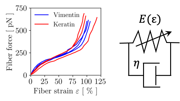
As a simple extension of the above case, we now consider modeling an elastic fiber with nonlinear modulus. According to the characteristic mechanical behavior often reported for intermediate filaments, we would like the modulus to comprise a softening regime, for values of the fiber strain ($\varepsilon_f = \frac{\ell}{\ell_0} - 1$) between $\varepsilon_f^{soften}$ and $\varepsilon_f^{stiffen}$, followed by a re-stiffening when $\varepsilon_f > \varepsilon_f^{restiffen}$. In terms of rheological elements, this yields a Kelvin-Voigt model where the spring modulus depends on the applied fiber strain.

Denoting with $E^{soften}$ and $E^{stiffen}$ the fiber moduli in the softening and re-stiffening regimes, we obtain:
$$ E \, (\varepsilon) = \begin{cases} E_0, & \text{if}\ \varepsilon < \varepsilon^{soften} \\ E^{soften} = E_0 \, \alpha^{soften}, & \text{if} \ \varepsilon^{soften} < \varepsilon < \varepsilon^{stiffen} \\ E^{stiffen} = E_0 \, \alpha^{stiffen}, & \text{if}\ \varepsilon > \varepsilon^{stiffen} \end{cases} $$where the ratios $\alpha^{soften}=E^{soften}/E_0$ and $\alpha^{stiffen}=E^{stiffen}/E_0$ have been introduced for convenience. Moreover, we ensure a gradual transition between the values of $E$ by reworking the above expression to reach:
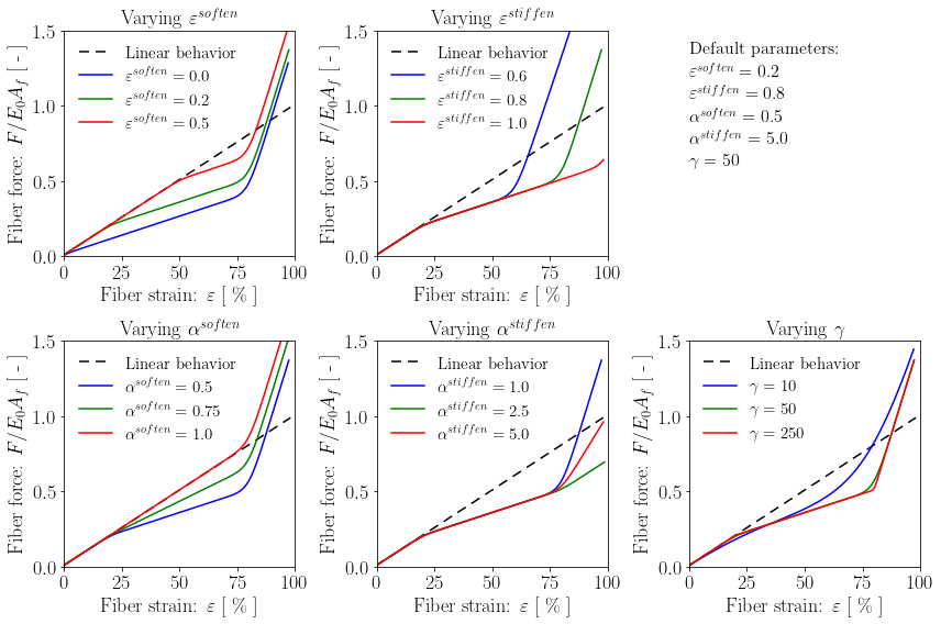
$$\frac{EA_f}{E_0A_f} \, (\varepsilon) = 1 + \frac{\alpha^{soften}-1}{1 + exp \left[-\gamma \left(\varepsilon-\varepsilon^{soften} \right) \right]} + \frac{\alpha^{stiffen}-\alpha^{soften}}{1 + exp \left[-\gamma \left(\varepsilon-\varepsilon^{stiffen} \right) \right]} $$where the scalar parameter $\gamma$ controls the smoothness of the transition between the different values of $E$.
In line with the previous sections, we also implement this fiber constitutive behavior in a Python function, which will now take the additional arguments EAfSoften, EAfStiffen, EpsSoften, EpsStiffen, and Gamma. To ensure $\tau \ll t_{load}$, we consider a constant retardation time and thus implicitly modify $\eta$ according to the values of $E$: $\eta(\varepsilon) = \tau \, E(\varepsilon)$.
def NonlinearKelvinVoigtFiber(ks, E0Af, EAfSoften, EAfStiffen, EpsSoften,\
                              EpsStiffen, Gamma, Tau, ell0, L, N, Tload):

    #pre-compute ratios of spring moduli
    alphaSoften  = EAfSoften  / E0Af
    alphaStiffen = EAfStiffen / E0Af

    #initialize arrays
    PQ    = ell0 * np.ones(N+1)      #values of PQ distance at each step
    ell   = ell0 * np.ones(N+1)      #values of fiber length at each step
    du_s  = np.zeros(N+1)            #values of current spring extension at each step
    f     = np.zeros(N+1)            #values of force acting at fiber ends at each step
    df    = np.zeros(N+1)            #change in force values from previous to current step (i.e. force step)
    EAf   = E0Af * np.ones(N+1)      #values of spring modulus at each step, multiplied by Af
    J_Af  = np.zeros(N+1)            #values of creep compliance function at each step, divided by Af
    eps   = np.zeros(N+1)            #values of fiber strain each step
    time  = np.linspace(0,Tload,N+1) #values of time at each step
    dT    = Tload / N                #time step

    #loop for load application
    for i in range(1,N+1):
        PQ[i]   = ell0 + i * (L - ell0) / N             #update current PQ distance
        du_s[i] = np.abs(PQ[i] - ell[i-1]) / 2.         #update current spring elongation
        f[i]    = ks * (PQ[i] - ell[i-1]) / 2.          #update current force at fiber ends
        df[i]   = f[i] - f[i-1]                         #update current force step
        EAf[i]  = E0Af * ( 1. + (alphaSoften-1.)/(1. + np.exp(-Gamma*(eps[i-1]-EpsSoften)))\
                          + (alphaStiffen-alphaSoften)/(1. + np.exp(-Gamma*(eps[i-1]-EpsStiffen))) )
                        #current EAf value
        for j in range(i):                              #update creep compliance function based on current time
            J_Af[j] = (1.0 - np.exp(-(time[i]-j*dT)/Tau))/EAf[j]
        eps[i]  = np.sum(J_Af*df)                       #determine fiber strain using Boltzmann's summation
        ell[i]  = eps[i] * ell0 + ell0                  #determine fiber length from current strain

    F = np.cumsum(df)                #measure force during loading as cumulative sum of the df values

    #return results
    return time, PQ, du_s, EAf, J_Af, ell, eps, F
Below we showcase the nonlinear elastic modulus provided by this function, and test the effect of varying the parameters EAfSoften, EAfStiffen, EpsSoften, EpsStiffen, and Gamma.

Modeling rate-dependent fiber stretchability using the standard linear solid model
The same approach that has allowed including a dashpot to dampen the fiber elongation can be leveraged to further enrich the fiber constitutive behavior. Below we consider the standard solid model in its Kelvin-Voigt representation, where a spring ($E_1$) is in series with the parallel of another spring ($E_2$) and a dashpot ($\eta_2$). Due to the peculiarities of our fiber loading algorithm, we additionally place a dashpot of viscosity $\eta_1$ in parallel to the first spring; this has the sole purpose of stabilizing the algorithm and thus we require that $\tau_1 = \eta_1/E_1 \ll t_{load}$ to mimize its influence on the mechanical response of the fiber.

Applying linear superposition, the creep compliance function becomes:
$$J(t) = \frac{1-e^{-t/\tau_1}}{E_1} + \frac{1-e^{-t/\tau_2}}{E_2}$$
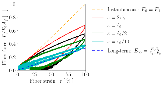
where $\tau_2 = \eta_2 / E_2$ controls the rate-dependent response of the fiber, as shown below using a modified Python function (not reported here for brevity):

Cytosim implementation and examples
We implement the constitutive behavior of a standard solid model in a dedicated Cytosim fiber class, which can be accessed through the keyword "activity = stretch" and takes the following parameters:
- rigidity $\rightarrow$ the fiber bending rigidity;
- segmentation $\rightarrow$ the fiber segmentation;
- constitutive $\rightarrow$ the coefficients of the standard solid model;
- nonlinear $\rightarrow$ the parameters governing the dependence of $E_1$ on the fiber strain.
Below we demonstrate the use of this fiber class by providing three examples.
Example 1: Modeling a linear elastic fiber behavior
In order to use "activity = stretch" to model the mechanical behavior of a fiber with linear elastic characteristics, we need to define two parameters using the keyword "constitutive":
- the product $EA_f$, between the fiber elastic modulus and its cross-sectional area, as first entry;
- the retardation time $\tau \ll t_{load}$ as a second entry, characterizing the Kelvin-Voigt model that we use to stabilize the fiber elongation algorithm.
Note that, when receiving only 2 entries to the keyword "constitutive", Cytosim automatically knows that we intend to use the Kelvin-Voigt model with constant spring modulus.
Assuming that we want to extend the fiber up to reaching twice its original length over a time period $t_{load} = 100$ s, we deem a value $\tau = t_{load}/80 = 1.25$ s as sufficiently small for the fiber to behave quasi-elastically. As indicated below, we also set $EA_f = 100$ pN, the initial fiber length to $\ell_0 = 10$ $\mu$m, the spring stiffness to $k_s = 1000$ pN / $\mu$m (so that $\gamma_0 = 100$), and adopt a simulation time step of $1$ ms:
cytosim
set fiber filament
{
     rigidity = 0.05
     segmentation = 0.2
     activity = stretch
     constitutive = 100, 1.25
     display = ( coloring = 1; )
}
new filament
{
     placement = none
     shape = -5.0 0 0, 5.0 0 0
}

set single clamp
{
     hand = bind
     activity = fixed
     stiffness = 1000.0
}
By running the stretching simulation included in the example file "stretch_fiberElastic.cym", we obtain the tensile behavior displayed below:

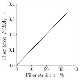
We confirm that the fiber behavior is linear and very close to perfect elasticity both for the case with $kT \sim 0$ (no Brownian motion) and for $kT > 0$.
Note that the above simulations require a large number of steps where the position of the clamps (i.e. points $P$ and $Q$) is modified. To avoid tedious manual operations associated with file generation, we provide a python function "generate.py" that allows automatically generating input files for simulations of fiber tensile loading. The function is found in ../cytosim/python/misc/ and can be used through the command "generate.py DEST_FOLDER", where DEST_FOLDER is the folder where the input file will be saved and the simulation parameters are directly defined in the file "generate.py".
Also note that the tensile behavior of a fiber can be conveniently extracted using the function "fiber:tensile" that is available using the "report" binary.
Example 2: Modeling a nonlinear elastic fiber behavior
To introduce a dependence of the fiber elastic modulus on the applied strain, we additionally need to provide the "nonlinear" parameters for a fiber with "activity = stretch". The required parameters are:
- the product $EA_f$ in the softening regime, $(EA_f)^{soften}$, as first entry;
- the product $EA_f$ in the re-stiffening regime, $(EA_f)^{stiffen}$, as second entry;
- the strain value at which the fiber softens, $\varepsilon^{soften}$, as third entry;
- the strain value at which the fiber re-stiffens, $\varepsilon^{stiffen}$, as fourth entry;
- the scalar parameter $\gamma$ as a fifth and last entry, characterizing the smoothness of the transition between regions with different fiber modulus.
cytosim
set fiber filament
{
     rigidity = 0.05
     segmentation = 0.2
     activity = stretch
     constitutive = 100, 1.25
     nonlinear = 50, 300, 0.2, 0.8, 50
     display = ( coloring = 1; )
}
new filament
{
     placement = none
     shape = -5.0 0 0, 5.0 0 0
}

set single clamp
{
     hand = bind
     activity = fixed
     stiffness = 1000.0
}
By running the stretching simulation included in the example file "stretch_fiberNonlinearElastic.cym", we obtain the nonlinear tensile behavior shown below. The deviation from elasticity is quite small and clearly due to the presence of the dashpot that is needed to stabilize the fiber elongation algorithm.

Example 3: Modeling a viscoelastic fiber behavior
We now consider a fiber that has constant constitutive parameters but features a time-dependent behavior. This can be modeled using the standard solid rheological model, which can be accessed by setting "activity = stretch" and providing the following entries via the keyword "constitutive":
- the product $E_1A_f$, between the elastic modulus $E_1$ and the fiber cross-sectional area, as first entry;
- the retardation time $\tau_1 \ll t_{load}$ as a second entry, which is needed to stabilize fiber mechanical response when this is dominated by the spring $E_1$;
- the product $E_2A_f$, between the elastic modulus $E_2$ and the fiber cross-sectional area, as third entry;
- the retardation time $\tau_2$ as a fourth entry, which dominates the rate-dependent behavior of the fiber.
Note that, when receiving all the 4 parameters associated with the keyword "constitutive", Cytosim is aware that we intend to use the complete standard solid model.
We simulate the same loading case as in Example 1 and set $E_2 = E_1/2$ and $\tau_2 = t_{load} = 100$ s:
cytosim
set fiber filament
{
     rigidity = 0.05
     segmentation = 0.2
     activity = stretch
     constitutive = 100, 1.25, 50, 100
     display = ( coloring = 1; )
}
new filament
{
     placement = none
     shape = -5.0 0 0, 5.0 0 0
}

set single clamp
{
     hand = bind
     activity = fixed
     stiffness = 1000.0
}
By running the stretching simulation included in the example files "stretch_fiberViscoElastic.cym", "stretch_fiberViscoElastic_2xFaster.cym", and "stretch_fiberViscoElastic_2xSlower.cym", we obtain a nonlinear and dissipative tensile behavior that depends on the rate of the applied deformation:

Similarly, we can simulate cyclic loading and observe how the tensile response of the fiber stabilizes:

Conclusions
We have discussed the implementation of longitudinal fiber extensibility in Cytosim and developed a custom fiber class that allows simulating the linear elastic, nonlinear elastic, and rate-dependent mechanical behavior of cytoskeletal fibers. This class can be accessed via the keyword "activity = stretch" and is modeled after other dedicated implementations of specific fiber behaviors that are available within Cytosim.